Estimating the Contribution of The Industrial Revolution to 20th Century Warming

Following is a rebuttal by John Abbot and me to claims that we misrepresent the Moberg et al. (2005) reconstruction of northern hemisphere temperatures over the last 2,000 years in our article published in GeoResJ in 2017.

1. Introduction

During the 12th Century, the English philosopher, diplomat and bishop, John of Salisbury (1120-1180) wrote that we see more and farther than our predecessors, not because we have keener vision or greater height, but because we are lifted-up and borne aloft on their knowledge.

When we undertook an analysis of the application of machine learning for evaluating anthropogenic versus natural climate change (Abbot and Marohasy 2017a), we did not claim to be experts on historical temperature reconstructions using proxy data. Rather we sought-out reconstructions by experts already published in the peer-reviewed scientific literature. Our contribution – building on this expert knowledge – was to show how the patterns in the temperature series could be decomposed into sine waves and then used as input into an artificial neural network (ANN) to generate a forecast.

Again, these are not new techniques or techniques that we invented. But this perhaps represents the first time ANNs – now routinely used in medical and driverless car research, for Google Translate, and in advertising and share market trading – have been applied to forecasting temperature using millennial-scale temperature reconstructions. There have been previous studies showing spectral analysis of long-term instrumental and proxy temperature records (e.g. Ludecke et al. 2013).

ANNs are a form of artificial intelligence (AI) and machine learning. Providing the ANN with the series as sine waves is a form of pre-processing, known as feature extraction. In essence, we were seeking to forecast the behaviour of the whole, by understanding its component parts. As long as the relationships embedded in the complex oscillation in the proxy-temperature series continue into the future, a skilful forecast is theoretically mathematically possible.

This was the hypothesis that we explicitly tested in this study published in GeoResJ (volume 14, pages 36-46): that there are natural climate cycles. This does not accord with the general consensus, which assumes that such cycles have been significantly perturbed by elevated levels of carbon dioxide since the Industrial Revolution. Of course, a key distinguishing feature of any scientific theory is that it is amenable to falsification, so it was valid for us to test this assumption, by way of hypothesis. Indeed, our article in GeoResJ (Abbot and Marohasy 2017a) tests a pillar of anthropogenic global warming theory by attempting to separate-out the contribution of the Industrial Revolution to 20th Century warming. We did this by forecasting the likely extent of warming in the absence of an Industrial Revolution using an ANN.

The article has been subject to considerable criticism particularly on the social media platform Twitter. Some of this criticism has been of our methodology, specifically the use of ANNs. Much of the criticism has been from climate scientists, and their followers, who are apparently only familiar with simulation modelling based on the coding of physical processes. To reiterate, our technique is widely applied to time-series data, for example, for forecasting in the financial sector.

It is the case that mainstream climate science relies exclusively on simulation models. For example, the IPCC relies on General Circulation Models including the Australian Bureau of Meteorology’s POAMA. Also the world’s most widely used atmospheric model, the Weather Research and Forecasting model is a simulation model. These models rely on the accurate simulation of physical processes, making various assumptions about the physics and chemistry of our oceans and atmosphere and incorporating carbon dioxide as a significant driver of climate change. Our GeoResJ article involved a completely different type of modelling, specifically the building of statistical models based on relationships inherent to the data using ANNs, while making no assumptions about physical processes.

Also, it has been claimed on Twitter that our article misrepresents the timeseries in one of the six proxy temperature series we deconstruct. Specifically, that our representation of Moberg et al. (2005) is incorrect because our series shows a shift of several decades along the time axis. Further it has been claimed that the crude digitisation of a timeseries is incompatible with rigorous analysis of data. We reject these criticisms, but only after evaluating each in some detail.

We begin this report with a consideration of northern hemisphere proxy temperature reconstructions by experts, because it is their treatment in the peer-reviewed technical literature, which underpins our study of the application of machine learning for evaluating anthropogenic versus natural climate change.

2. Proxy Temperature Reconstructions for the Northern Hemisphere

The 12th Century was a period of general optimism in Europe that corresponded with what Moberg et al. (2005) describe as a warm peak around AD 1100, followed by pronounced coolness in the sixteenth and seventeenth centuries (page 615). History books often refer to this as the Medieval Warm Period (MWP), which was followed by the Little Ice Age (LIA). The end of the LIA corresponds with the beginning of industrialization, but this correlation may not involve causation. Whether industrialization actually caused the end of the LIA, and the beginning of a period of warming, is a valid hypothesis. It is also valid to ask the question: to what extent may natural climate cycles have been perturbed by the Industrial Revolution.

The two periods (the MWP and LIA) are generally evident in reconstructions of millennial-scale climate variability for the northern hemisphere, for example in the first IPCC assessment report (Houghton et al. 1991), and more recently, for example, in Wilson et al (2016). However, since the publication of Mann et al. (1999), and the prominence of this northern hemisphere reconstruction in chapter 2 of the IPCC’s third assessment report, there has been controversy associated with these reconstructions.

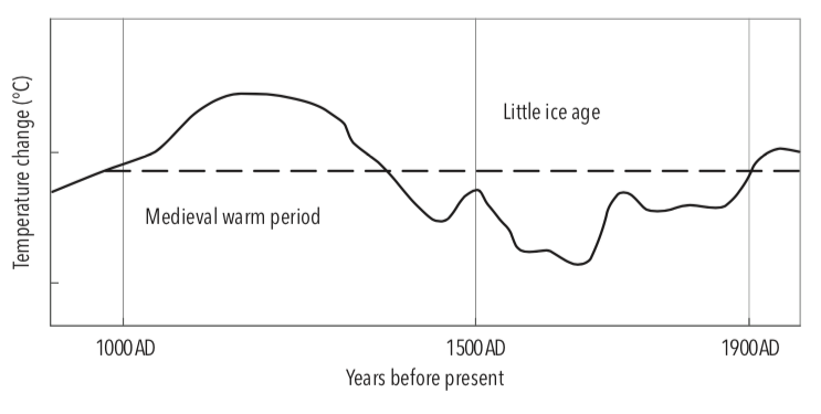
Chart 1. Schematic diagram of global temperature variations during the last thousand years as shown on page 202 of the IPCC Scientific Assessment published in 1991.

Chart 2. The ‘hockey stick’ as shown in chapter 2, Climate Change 2001: The Scientific Basis, in the IPCC Third Assessment Report.

Moberg et al. (2005) is an often-cited reconstruction of northern hemisphere temperatures for the past 2,000 years, that attempts to address some of the controversy. Moberg et al. (2005) incorporates reference to the reconstructions in Mann and Jones (2003) and Mann et al. (1998). The Moberg et al. (2005) manuscript explains how to combine low-resolution proxies – such as interpretations of past temperature from stalagmites, boreholes, and also pollen, shells and diatoms in lake sediments – with high-resolution tree-ring data.

The Moberg et al. article as published in Nature is supported by supplementary information, which can be downloaded from www.nature.com/nature. This includes seven time series for tree-ring data as ‘Supplementary Figure 2’. In the actual article, there is a low-frequency reconstruction that shows borehole data to the year 1990 (Figure 2d, page 616). There is also a calibrated reconstruction (Figure 2b). But it is difficult to see the pattern of temperature change in this series from about 1900 (red line), because it has been overlaid with an instrumental temperature series (green line): as shown in Chart 3 of this report.

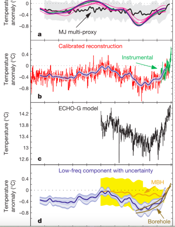
Chart 3. These are the temperature series shown in Moberg et al. 2005 as published in Nature, volume 433. The red line at b is the proxy temperature reconstruction, which has been obscured by the imposition of a homogenized instrumental temperature series (green), and other representations (blue).

Geirsdottir et al. (2009) includes a time series cited as Moberg et al. (2005), that is not overlaid with an instrumental series, and extends to the year 2000, labelled Figure 13E – and shown in this report in Chart 4. Furthermore, the high frequency variability in the Moberg series (the red line in Figure 2b, shown here in Chart 3) is smoothed by Geirsdottir et al. 2009, presumably by taking a moving average. This is a common technique in climate science, used to reduce the ‘noise’ in such series.

Geirsdottir et al. (2009) is one of 14 articles published in a special issue of the Journal of Paleolimnology. The journal has been published for nearly 40 years and is a major repository for articles dealing with climate change. The special edition which includes Gerisdottir et al. (2009) was dedicated to Holocene climate change and was edited by Darrell Kaufman. Dr Kaufman manages a large research unit that specializes in proxy climate records.

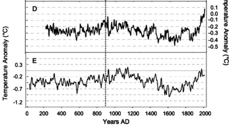
Chart 4. This is an extract from Figure 13 of Geirsdottir et al. 2009 as published by the Journal of Paleoliminology, volume 41. The series at E is cited as “Moberg et al. (2005) reconstructed Northern Hemisphere temperatures calculated by combining low-resolution proxies with tree-ring data, using a wavelet transform technique to achieve timescale-dependent processing of the data”.

3. Using Digitized Values from Published Graphical Temperature Proxy Reconstructions

For our assessment of the application of machine learning for evaluating natural versus anthropogenic climate change we choose to use values which in every instance were digitized using UN-SCAN-IT software, specifically we digitized published graphical temperature proxy reconstructions. This is explained in the second paragraph of the ‘Methods’ section of our article (page 37).

While it may have been preferable to use the actual values for each of the six series that we deconstructed in our GeoResJ article, very few journals currently make the archiving of such values mandatory – and authors are under no obligation to provide such data when they receive requests, as illustrated by our failed request to Aslaug Giersdottir (see Section 4 of this report).

We have previously had difficulty accessing actual values used to support the conclusions of published studies, and we have published on this issue including in a series of articles in Environmental Law and Management (Abbot and Marohasy 2010 a, b and 2012 a).

In the final assessment, scanning graphical representations is a valid approach because it is a way of obtaining the coordinates of interest from published studies.

4. Comparing Giersdottir et al. 2009 with Moberg et al. 2005

In our GeoResJ article, we cite Giersdottir et al. (2009), not Moberg et al. (2005) as the source of our northern hemisphere proxy reconstruction. Yet it has been claimed that this is an incorrect representation of Moberg et al. (2005), specifically that we have shifted the time-series. We have so far not been accused of incorrectly representing Giersdottir et al. (2009), whose depiction of Moberg et al. (2005) has not been criticized.

We wrote to Aslaug Giersdottir on 28th April 2018 asking for the actual numbers used in the construction of the chart shown as Figure 13E, and the source of these values that is cited as Moberg et al. 2005. Dr Geirsdottir has never responded. We have since been provided with access to a set of tabulated numbers for Moberg et al. 2005,
available at ftp://ftp.ncdc.noaa.gov/pub/data/paleo/contributions_by_author/moberg2005/nhtemp-moberg2005.txt .

We have plotted these values from this NOAA archive, with the digitized values from Figure 13E in Giersdottir et al (2009), as shown in Chart 5.

It is apparent that while the Moberg et al. (red) and Geirsdottir et al. (black) series follows a similar pattern, Moberg et al. (2005) could be characterized as noisier, and Geirsdottir et al. (2009) does not correspond to a simple displacement of the Moberg et al. series.

It is not clear to us how Geirsdottir et al. (2005) derived the values from Moberg et al. (2005), and our correspondence requesting clarification has never been answered. But there is no reason to believe that the Geirsdottir chart was exclusively derived from the tabulated annual data as shown in our Chart 5. It is quite conceivable that Figure 13E in Geirsdottir et al. 2009 was constructed from other supplementary data provided by Anders Moberg.

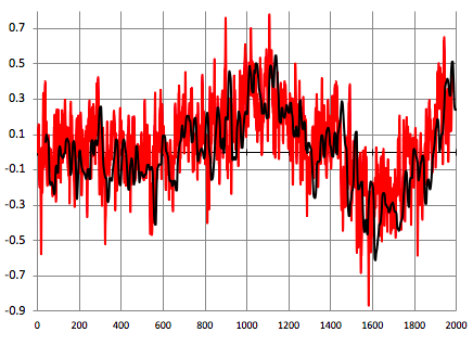
Chart 5. Tabulated annual values for Moberg et al. (2005) as downloaded from the NOAA website, with Geirsdottir et al. (2009) at E in Figure 13 as digitized using UN-SCAN-IT software.

It is common in climate science for important time-series to be added onto. For example, in our work forecasting monthly rainfall (e.g. Abbot and Marohasy 2014) we use a climate index known as the Interdecadal Pacific Oscillation (IPO), which is regularly updated by Chris Folland formerly of the UK Met Office, and he requests Power et al. (1999) be cited as the source for the series. As a further example, the KNMI Climate Explorer website supported by the Dutch Met Office and the World Meteorological Organisation, provides values for Nino 3.4 updated to October 2018 (at the time of writing), and indicates that the reference is Huang et al. 2017. Indeed, when downloading up-to-date series at various online websites hosted by government research institutions there is often the name of a publication that users of the downloadable series are requested to cite.

5. Calculating temperature deviations based on Moberg et al. tabulated values

One measure of the robustness of our approach is to see if it withstands replication. Specifically, if we use the tabulated values for Moberg et al. (2005) as downloadable from the NOAA website – rather than the digitised values we generated from Geirsdottir et al. (2009) –
will we get the same answer?

In our original study, published in GeoResJ, we took the digitised time-series and submitted them to spectral analysis using Autosignal software. In each case the number of sine curves applied to reconstruct the pattern in the series was increased until the improvement in fitting, estimated by correlation coefficient, showed only marginal improvement. By adjustment of periodicities, phase and power of the identified sine wave components, the software optimises simulations of the original proxy signal, using a defined number of component sine waves. The optimization was undertaken from the proxy-temperature series start date through until 1830, as this is regarded as the pre-industrial period.

In this new study, detailed here for the first time, the Moberg et al. (2005) tabulated values were used, as well as moving averages derived from this data, specifically of 10, 20, 30 and 40 years.

These series are shown as the red lines in Charts 6, 7, 8, 9 and 10. The charts also show the ANN-derived series as the green line. Specifically, the green line after 1880 is the temperature forecast. Because the forecast is derived from a pre-industrial ‘training period’ (to use the language of machine learning), the forecast is of temperatures assuming no perturbance from elevated levels of carbon dioxide.

We calculated the average difference between the proxy temperatures as shown by the red lines and the forecast temperatures as shown by the green line (ANN-derived) to determine the deviation. These values are shown in Table 1. They range from 0.20 to 0.03. The values in our original study ranged from 0.20 to 0.06: Table 12 (page 40) as published in GeoResJ.

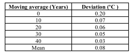
Table 1. Deviation between proxy temperature series from Moberg et al. (2005) and ANN forecast for the period 1880 to 1980.

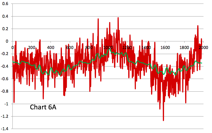
Chart 6A. Proxy temperature record (red) and artificial neural network output (green), based on Moberg et al. (2005).
ftp://ftp.ncdc.noaa.gov/pub/data/paleo/contributions_by_author/moberg2005/nhtemp-moberg2005.txt .

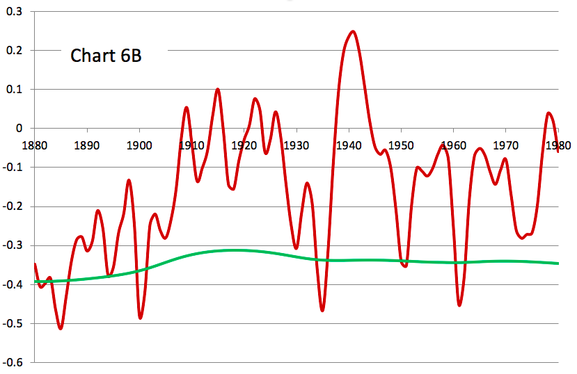
Chart 6B. Proxy temperature record (red) and artificial neural network output (green), only showing the forecast period 1880 to 1980.

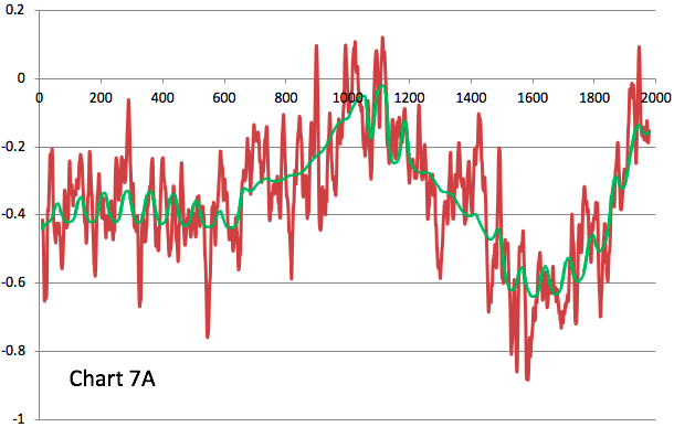
Chart 7A. Proxy temperature record (red) and artificial neural network output (green), based on Moberg et al. (2005) smoothed with a 10-year moving average.
ftp://ftp.ncdc.noaa.gov/pub/data/paleo/contributions_by_author/moberg2005/nhtemp-moberg2005.txt .

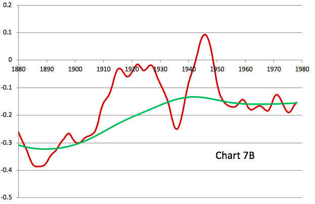
Chart 7B. Proxy temperature record (red) and ANN output (green) from Moberg et al. (2005) smoothed with a 10-year moving average, only showing the forecast period 1880 to 1980.

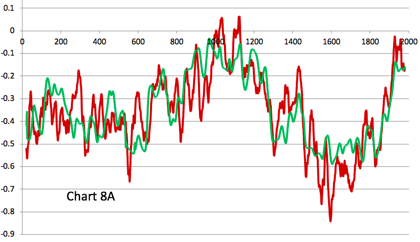
Chart 8A. Proxy temperature record (red) and artificial neural network output (green), based on Moberg et al. (2005) smoothed with a 20-year moving average.
ftp://ftp.ncdc.noaa.gov/pub/data/paleo/contributions_by_author/moberg2005/nhtemp-moberg2005.txt .

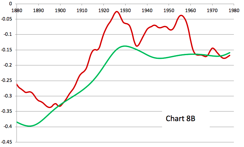
Chart 8B. Proxy temperature record (red) and ANN output (green) from Moberg et al. (2005) smoothed with a 20-year moving average, only showing the forecast period 1880 to 1980.

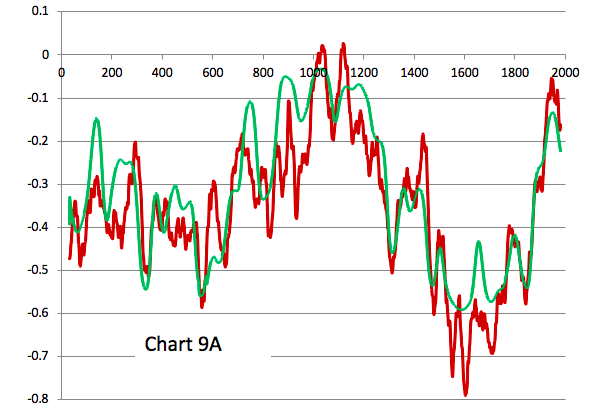
Chart 9A. Proxy temperature record (red) and artificial neural network output (green), based on Moberg et al. (2005) smoothed with a 30-year moving average.
ftp://ftp.ncdc.noaa.gov/pub/data/paleo/contributions_by_author/moberg2005/nhtemp-moberg2005.txt .

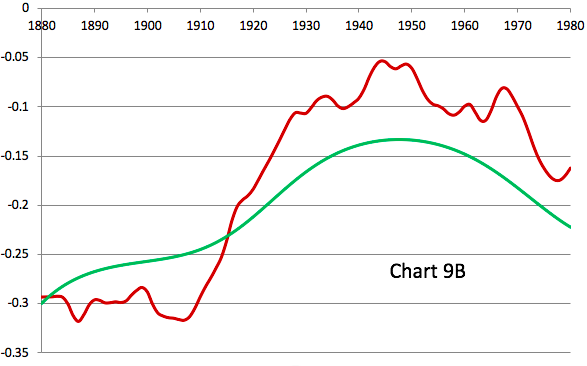
Chart 9B. Proxy temperature record (red) and ANN output (green) from Moberg et al. (2005) smoothed with a 30-year moving average, only showing the forecast period 1880 to 1980.

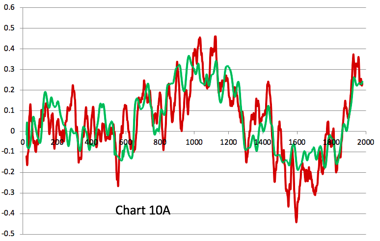
Chart 10A. Proxy temperature record (red) and artificial neural network output (green), based on Moberg et al. (2005) smoothed with a 40-year moving average.
ftp://ftp.ncdc.noaa.gov/pub/data/paleo/contributions_by_author/moberg2005/nhtemp-moberg2005.txt .

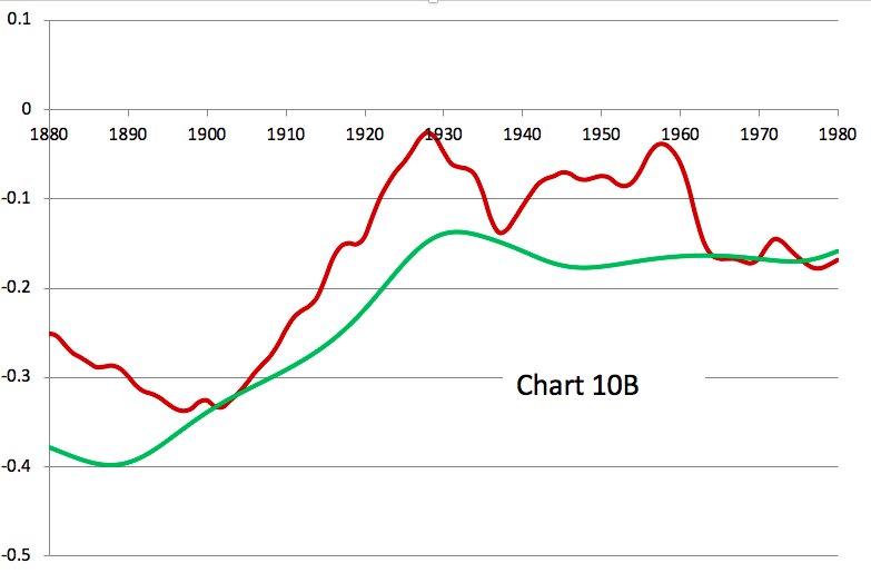
Chart 10B. Proxy temperature record (red) and ANN output (green) from Moberg et al. (2005) smoothed with a 40-year moving average, only showing the forecast period 1880 to 1980.

Importantly, the temperature deviations that we calculated from the Moberg et al. (2005) tabulated values, all lie in a range below the maximum values previously reported in Table 12 of Abbot and Marohasy (2017a). To be clear, whether using the Geirsdottir et al. (2009) version of Moberg et al. (2005) as we did in our article in GeoResJ, or the tabulated values archived at the NOAA website, or series derived from various moving-averages, the deviation is no more than 0.2 degrees Celsius.

6. In conclusion

We do not claim to be experts on the reconstruction of millennial-scale temperature series, or the archiving of such proxy temperature data. Rather we have spent some years learning how to apply the latest developments in artificial intelligence (AI), specifically artificial neural networks (ANNs), for forecasting monthly rainfall (Abbot and Marohasy 2012b, Marohasy and Abbot 2015, Abbot and Marohasy 2016, Abbot and Marohasy 2017b, etc.).

In putting together arrays for forecasting monthly rainfall, we rely on input variables that variously include local rainfall, land surface temperatures, sea surface temperatures and pressures across the Pacific Ocean, sea surface temperatures for the north-western Indian Ocean, and also sunspot cycles. Some of these series are presented as climate indices that we routinely download from the KNMI Climate Explorer website supported by the Dutch Met Office and the World Meteorological Organisation. We could not generate skillful monthly rainfall forecasts without access to these climate indices. In short, we build-on the knowledge of others.

In our first study forecasting proxy temperatures, we used digitised versions of proxy temperature series from graphical representations in published studies that extend to the year 2000. We trusted that a series in a special issue of the Journal of Paleoliminology, clearly presented as a temperature anomaly, at a scale and resolution suitable for our purposes, extending to the year 2000, was an accurate representation of past temperatures for the northern hemisphere.

After it was drawn to our attention that this series is a variation of Moberg et al. (2005), and after we were provided with tabulated values from Moberg et al. (2005) which only extends to 1980, we subjected this data to the same analysis.

We took the tabulated values, as well as moving-averages of 10, 20, 30 and 40-years. Each series was decomposed into sets of sine waves and then we used an ANN to generate forecasts of proxy temperatures for the period 1880 to 1980. Finally, we calculated the average deviation between the proxy temperature tabulated values and the ANN forecast as an estimation of natural climate change assuming no Industrial Revolution. That is, the divergences between our forecasts from the ANN (green line) and the proxy series based on Moberg et al. (2005) (red line) in Charts 6B, 7B, 8B, 9B and 10B, was used as an indication of the extent of human-caused warming in the northern hemisphere between 1880 and 1980.

Importantly, the temperature deviations that we calculated from this new analysis (using the tabulated values from Moberg et al. 2005) is no more than 0.2 degrees Celsius. Based on the rational in our original published study in GeoResJ (specifically knowing the corresponding rise in atmospheric carbon dioxide levels over this period) we again estimate an Equilibrium Climate Sensitivity (ECS) of approximately 0.6 degrees Celsius.

7. References

Abbot J. & Marohasy J. 2010a. Accessing environmental information relating to climate change: a case study under UK freedom of information legislation. Environmental Law and Management, 22 (1), 3- 12.

Abbot J. & Marohasy J. 2010b. Accessing information relating to climate change: the case of Irish oaks tree rings. Environmental Law and Management, 22 (4), 172-181.

Abbot J. & Marohasy J. 2012a. Accessing information under Australian freedom of information legislation: a case study involving climate change. Environmental Law and Management, 24 (3), 114-118

Abbot J. & Marohasy J. 2012b. Application of artificial neural networks to rainfall forecasting in Queensland, Australia. Advances in Atmospheric Sciences, 29 (4), 717-730. doi: 10.1007/s00376-012-1259-9

Abbot J. & Marohasy J. 2014. Input selection and optimisation for monthly rainfall forecasting in Queensland, Australia, using artificial neural networks. Atmospheric Research, Volume 138, Pages 166-178.

Abbot J. & Marohasy J. 2016. Forecasting monthly rainfall in the Bowen Basin of Queensland, Australia, using neural networks with Nino indices. In AI 2016: Advances in Artificial Intelligence, Eds. B.H. Kand & Q. Bai. DOI: 10.1007/978-3-319-50127-7_7.

Abbot J. & Marohasy J. 2017a. The application of machine learning for evaluating anthropogenic versus natural climate change, GeoResJ 14, 36-46. http://dx.doi.org/10.1016/j.gf.2017.08.001

Abbot J. & Marohasy, J. 2017b. Skilful rainfall forecasts from artificial neural networks with long duration series and single-month optimisation, Atmospheric Research 197, 289-299. DOI10.1016/j.atmosres.2017.07.01

Geirsdottir A. Miller G. Thordarson T. et al. 2009. A 2000 year record of climate variations reconstructed from Haukadalsvatn, West Iceland, Journal of Paleolimnology 41, 95-115.

Houghton JT, Jenkins GJ, Ephraums JJ. 1991. The IPCC Scientific Assessment, Cambridge University Press, MA.

Huang B. Thorne, PW. Banzon, VF. et al. 2017. Extended Reconstructed Sea Surface Temperatures Version 5 (ERSSTv5): Upgrades, Validations, and Intercomparisons. Journal of Climate, https://doi.org/10.1175/JCLI-D-16-0836.1

Lüdecke HJ, Hempelmann A, &Weiss CO. 2013. Multi-periodic climate dynamics: spectral analysis of long-term instrumental and proxy temperature records, Climate of the Past, 9, 447-452

Mann ME, Bradley RS & Hughes MK. 1998. Global-Scale Temperature Patterns and Climate Forcing Over the Past Six Centuries, Nature, 392, 779-787.

Mann ME, Bradley RS & Hughes MK. 1999.Northern hemisphere temperatures during the past millennium: Inferences, uncertainties, and limitations. Geophysical Research Letters 26, 759-762.

Mann ME, Jones PD 2003. Climate over past millennia, Geophysical Research Letters 30, 1820.

Marohasy J. & Abbot J. 2015. Assessing the quality of eight different maximum temperature time series as inputs when using artificial neural networks to forecast monthly rainfall at Cape Otway, Australia, Atmospheric Research 166, 141-149. doi: 10.1016/j.atmosres.2015.06.025.

Moberg A. Sonechkin DM. Holmgren K. et al. 2005. Highly variable Northern Hemisphere temperatures reconstructed from low- and high-resolution proxy data, Nature 433, 613-617.

Power S. Casey T. Folland C. et al., 1999: Inter-decadal modulation of the impact of ENSO on Australia. Climate Dynamics, 15, 319-323.

Wilson R. Anchukaitis K. Briffa K. et al. 2016. Last millennium northern hemisphere summer temperatures from tree rings: Part 1: The long term context. Quaternary Science Reviews 134,1-18.